Overall architecture

Block diagrams
| (Baseline) ATT-MVDR |
|---|

|
| (Proposed) SB-ATT-MVDR |

|
Model architectures
| MC-MaskNet (Multi-Channel Mask Estimation Network) |
|---|

|
Comparison of attention-based SCM estimation methods

All three build the same masked instantaneous SCM \(\mathbf{\Psi}^{\nu}(t,f)=m^{\nu}(t,f)\mathbf{Y}\mathbf{Y}^{\mathsf H}\) and feed the same Souden MVDR filter. They differ only in how \(\mathbf{\Psi}\) is aggregated into \(\mathbf{\Phi}\).
- Stage 1, group the bins. ATT-MVDR and NL-ATT-MVDR use one full-band group; SB-ATT-MVDR uses 32 subbands.
- Stage 2, flatten the instantaneous SCMs. ATT-MVDR and NL-ATT-MVDR produce 25,650 real values per frame; SB-ATT-MVDR produces 400, 800 or 1,600 per subband.
- Stage 3, project. ATT-MVDR and NL-ATT-MVDR project to 256 dimensions; SB-ATT-MVDR projects to 100 and shares one projection across subbands of equal width.
- Stage 4, encode. ATT-MVDR uses six Transformer layers of width 256; NL-ATT-MVDR uses two of width 256; SB-ATT-MVDR uses two of width 100. All use four attention heads.
- Stage 5, make the weights. ATT-MVDR produces one T by T matrix; NL-ATT-MVDR produces none and predicts the SCM directly; SB-ATT-MVDR produces one matrix per subband.
- Stage 6, aggregate. ATT-MVDR reuses one matrix at every frequency; SB-ATT-MVDR applies the matrix of the subband that owns the bin.
- SCM estimator parameters: 29.2 million, 31.8 million, and 1.4 million respectively; with the shared 1.28 million-parameter MC-MaskNet mask estimator the complete systems are 30.5, 33.1 and 2.7 million.
| Stage | ATT-MVDR | NL-ATT-MVDR | SB-ATT-MVDR proposed |
|---|---|---|---|
| 1 · Group the bins | All \(F\) bins at once 1 group |
Split into subbands \(\mathcal{F}_n\), \(G_n\) bins each \(N=32\) groups |
|
| 2 · Flatten the ISCMs | \(\psi^{\nu}(t)\in\mathbb{R}^{2FC^{2}}\) 25,650 values |
\(\psi_n^{\nu}(t)\in\mathbb{R}^{2G_nC^{2}}\) 400 / 800 / 1,600 values |
|
| 3 · Project | \(E^{\nu,0}=\mathrm{Linear}(\psi^{\nu})\) → \(\mathbb{R}^{256}\) |
\(E_n^{\nu,0}=\mathrm{Linear}_n(\psi_n^{\nu})\), shared per \(G_n\) → \(\mathbb{R}^{100}\) |
|
| 4 · Encode | \(E^{i}=\mathrm{Encoder}^{i}(E^{i-1})\) \(D=256\), \(I=6\), 4 heads |
\(E^{i}=\mathrm{Encoder}^{i}(E^{i-1})\) \(D=256\), \(I=2\), 4 heads |
\(E_n^{i}=\mathrm{Encoder}^{i}(E_n^{i-1})\) \(D=100\), \(I=2\), 4 heads |
| 5 · Make the weights | \(\mathbf{A}=\mathrm{Softmax}\!\left(\tfrac{QK^{\mathsf T}}{\sqrt{D^{K}}}\right)\) \(\mathbb{R}^{T\times T}\) — one matrix |
none — the SCM is predicted directly no \(\mathbf{A}\) |
\(\mathbf{A}_n^{\nu}\) from the subband embeddings \(\mathbb{R}^{N\times T\times T}\) — one per subband |
| 6 · Aggregate | \(\mathbf{\Phi}^{\nu}(t,f)=\sum_{t'}A^{\nu}(t,t')\mathbf{\Psi}^{\nu}(t',f)\) same \(\mathbf{A}\) at every \(f\) |
\(Z=\mathrm{Linear}(E^{I})\), \(\mathbf{\Phi}=\mathrm{Reshape}(Z)\) no weighted sum |
\(\mathbf{\Phi}^{\nu}(t,f)=\sum_{t'}A_{n}^{\nu}(t,t')\mathbf{\Psi}^{\nu}(t',f),\; f\in\mathcal{F}_n\) weights follow the subband |
| SCM estimator parameters | 29.2 M 30.5 M with MC-MaskNet |
31.8 M 33.1 M with MC-MaskNet |
1.4 M 2.7 M with MC-MaskNet |
Full symbol list
| Symbol | Meaning |
|---|---|
| \(t,\ t'\) | Output (query) frame and contributing (key) frame; \(T\) frames total |
| \(f,\ F\) | One-sided STFT bin index and count |
| \(C\) | Microphone count (5) |
| \(\nu\) | Source label: desired speech (S) or noise (N) |
| \(m^{\nu}(t,f)\) | Mask from the mask estimator |
| \(\mathbf{\Psi}^{\nu},\ \mathbf{\Phi}^{\nu}\) | Instantaneous and aggregated SCM, \(C\times C\) |
| \(A^{\nu}(t,t')\), \(A_n^{\nu}(t,t')\) | Contribution of frame \(t'\) to the SCM at frame \(t\); shared across all bins (ATT-MVDR) or specific to subband \(n\) (SB-ATT-MVDR) |
| \(D,\ I\) | Embedding width and encoder layer count |
| \(n,\ N,\ G_n,\ \mathcal{F}_n\) | Subband index, count, bins per subband, and its bin set |
Experimental Setup
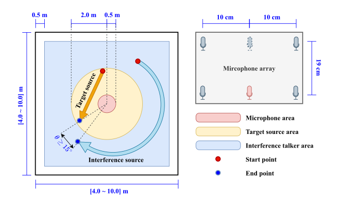
Detailed model / dataset configurations referenced from the paper. Simulation uses gpuRIR with WSJ0 speech, CHiME-3 noise, and a moving competing talker.
| Item | Value |
|---|---|
| Model configuration | |
| No. of Transformer-encoder layers | 2 |
| No. of attention heads | 4 |
| Dim. of Transformer-encoder layers | 100 |
| Dim. of feedforward layer | 800 |
| Sample rate | 16 kHz |
| Window / FFT / Hop | Hann / 1024 / 256 |
| Dataset configuration | |
| Room width [Lx] (m) | [4.0, 10.0] |
| Room depth [Ly] (m) | [4.0, 10.0] |
| Room height [Lz] (m) | [2.5, 4.0] |
| Speech corpus | WSJ0 |
| Noise corpus | CHiME-3 |
| No. of microphones | 5 |
| No. of sources / interferers | 1 / 1 |
| RT60 (s) | [0.1, 0.3] |
| Trajectory points | 128 |
| Height of mic / source (m) | 1.0 / [1.5, 1.9] |
| No. of data [train, val, test] | [30000, 2000, 2000] |
| Target-to-interference-plus-noise ratio, SINR (dB) | [0, 10] |
| Interferer-to-diffuse-noise ratio, INR (dB) | [-10, 10] |
Additional simulation details: minimum angular separation 15°; target distance 0.5–2.0 m from the array center, interferer at least 2.0 m; interferer-to-diffuse-noise SNR in [-10, 10] dB. Training uses Adam with early stopping (up to 200 epochs, batch size 24); oracle Wiener-like masks for ISCM computation during training, and estimated masks at inference.
Implementation Details
STFT and channel settings
| Item | Value |
|---|---|
| Sampling rate | 16 kHz |
| Window | Hann, length 1024 |
| FFT size / hop | 1024 / 256 (75% overlap) |
| Microphones | 5 of the 6 recorded channels, zero-based indices 0, 2, 3, 4, 5 |
| Reference channel | 4th of the 0, 2, 3, 4, 5 channels |
| Diagonal loading | 1e-6 · I added to the noise SCM before inversion |
| Algorithmic latency | Whole utterance (non-causal) |
These STFT settings are those used by all ATT-MVDR variants, including the proposed SB-ATT-MVDR. ABIC-MVDR and EaBNet follow their own published front ends.
SCM estimator configurations
| Item | ATT-MVDR | NL-ATT-MVDR | SB-ATT-MVDR (proposed) |
|---|---|---|---|
| Explicit temporal weight matrix | Yes, one T×T matrix shared by every frequency bin | No — the SCM is predicted directly, with no weighted sum of input ISCMs | Yes, one T×T matrix per subband |
| Embedding dim dmodel | 256 | 256 | 100 |
| Feed-forward dim | 2048 | 2048 | 800 |
| Attention heads | 4 | 4 | 4 |
| Encoder layers I | 6 | 2 | 2 |
| ISCM projection | Single full-band linear | Direct SCM projection | One linear layer per \(G_n\), shared by the subbands of that size |
| Subband partition | — | — | N = 32 subbands: Gn = 8, 16 and 32 for 16, 8 and 8 subbands, covering 0–2, 2–4 and 4–8 kHz respectively |
| Mask estimator (MC-MaskNet) | 1.28 M | 1.28 M | 1.28 M |
| SCM estimators (speech + noise) | 29.2 M | 31.8 M | 1.4 M |
| Complete system (mask + SCM) | 30.5 M | 33.1 M | 2.7 M |
Training objective
Every compared system except EaBNet minimised the scale-dependent SNR loss below, so the beamforming comparison is not confounded by the objective. EaBNet instead used its original combined spectral-magnitude and real–imaginary MSE loss.
L = −10 log10 ( ‖s‖2 / ‖s − ŝ‖2 )
| Symbol | Meaning |
|---|---|
| s | Time-domain target speech |
| ŝ | Estimated speech: the beamformed output converted back to the time domain by the inverse STFT |
| ‖·‖ | L2 norm |
Quantitative Performance Evaluation
| Model | Param. (M) | GMAC/s | PESQ-nb | PESQ-wb | STOI | BSS-SDR (dB) | WER (%) |
|---|---|---|---|---|---|---|---|
| Noisy | - | - | 1.90 | 1.34 | 0.83 | 4.93 | 5.54 |
| ConvTasNet | 8.8 | 2.84 | 2.91 | 2.30 | 0.93 | 13.35 | 6.13 |
| - NL-ATT-MVDR | 40.6 | 4.87 | 3.15 | 2.63 | 0.95 | 15.45 | 4.83 |
| - ATT-MVDR | 38.0 | 4.73 | 2.98 | 2.58 | 0.95 | 15.98 | 3.68 |
| - IC-ATT-MVDR | 40.6 | 4.87 | 3.13 | 2.66 | 0.95 | 15.41 | 4.29 |
| - SB-ATT-MVDR | 10.2 | 5.01 | 3.17 | 2.73 | 0.96 | 16.17 | 3.88 |
| ABIC-MVDR | 0.35 | 4.01 | 3.20 | 2.78 | 0.97 | 16.68 | 2.64 |
| EaBNet | 2.83 | 7.35 | 3.28 | 2.86 | 0.97 | 16.54 | 2.49 |
| MC-MaskNet | 1.28 | 3.04 | 3.35 | 2.84 | 0.96 | 15.58 | 2.56 |
| - NL-ATT-MVDR | 33.1 | 5.11 | 3.42 | 2.96 | 0.97 | 17.21 | 2.51 |
| - ATT-MVDR | 30.5 | 4.98 | 3.16 | 2.82 | 0.97 | 17.29 | 2.50 |
| - IC-ATT-MVDR | 33.1 | 5.11 | 3.37 | 2.95 | 0.97 | 16.97 | 2.46 |
| - SB-ATT-MVDR | 2.7 | 5.25 | 3.34 | 2.97 | 0.97 | 17.42 | 2.44 |
| Model | PESQ-nb | PESQ-wb | STOI | BSS-SDR (dB) | WER (%) |
|---|---|---|---|---|---|
| Noisy | 1.90 | 1.34 | 0.83 | 4.93 | 5.54 |
| EaBNet | 3.13 | 2.71 | 0.96 | 16.05 | 2.57 |
| ABIC-MVDR | 3.17 | 2.73 | 0.96 | 16.02 | 2.56 |
| MC-MaskNet | 3.27 | 2.75 | 0.96 | 15.32 | 2.69 |
| - NL-ATT-MVDR | 3.35 | 2.89 | 0.97 | 16.91 | 2.59 |
| - ATT-MVDR | 3.05 | 2.62 | 0.96 | 15.98 | 2.52 |
| - IC-ATT-MVDR | 3.29 | 2.85 | 0.97 | 16.62 | 2.57 |
| - SB-ATT-MVDR | 3.27 | 2.86 | 0.97 | 16.84 | 2.48 |
Causal models apply an upper-triangular mask to the temporal attention, so frame \(t\) attends only to frames \(\le t\) with zero lookahead, and the mask estimator uses cumulative layer normalisation instead of instance normalisation.
| Local-SINR range | Mean | Target gain | Noise gain | ||||
|---|---|---|---|---|---|---|---|
| ATT | NL | SB | ATT | NL | SB | ||
| < -10 dB | -23.31 | -2.07 | -6.10 | -3.39 | -19.87 | -20.79 | -23.63 |
| [-10, 0) dB | -5.03 | -1.51 | -2.53 | -1.59 | -12.44 | -10.55 | -13.31 |
| [0, 10) dB | 4.81 | -0.93 | -0.69 | -0.71 | -10.26 | -6.63 | -10.05 |
| ≥ 10 dB | 20.08 | -0.22 | +0.01 | -0.11 | -7.07 | -3.33 | -6.58 |
Values are in dB. Target gains closer to 0 dB indicate better preservation, whereas lower noise gains indicate stronger suppression.
| Model | PESQ-nb | PESQ-wb | STOI | BSS-SDR (dB) | WER (%) |
|---|---|---|---|---|---|
| Noisy | 1.90 | 1.34 | 0.831 | 4.93 | 5.54 |
| ATT-MVDR | 3.27 | 2.98 | 0.974 | 17.64 | 2.31 |
| NL-ATT-MVDR | 3.67 | 3.32 | 0.980 | 18.37 | 2.20 |
| SB-ATT-MVDR | 3.74 | 3.47 | 0.984 | 19.02 | 2.29 |
| Model | Gn | Ranges | N | Shared FC layer | Param. (M) | GMAC/s | PESQ-wb | STOI | WER (%) |
|---|---|---|---|---|---|---|---|---|---|
| Noisy | - | - | - | - | - | - | 1.34 | 0.83 | 5.54 |
| ATT-MVDR | All | [8] | 1 | - | 30.5 | 4.97 | 2.82 | 0.97 | 2.50 |
| V1 | [4, 8, 32, 64] | [1, 3, 6, 8] | 40 | Yes | 3.2 | 5.71 | 2.95 | 0.97 | 2.51 |
| V2 | [4, 32, 64] | [2, 4, 8] | 40 | Yes | 3.1 | 5.71 | 2.92 | 0.97 | 2.50 |
| V3 | [4, 8, 64] | [1, 4, 8] | 44 | Yes | 2.9 | 5.94 | 2.96 | 0.97 | 2.49 |
| V4 | [32] | [8] | 16 | Yes | 2.4 | 4.33 | 2.89 | 0.97 | 2.52 |
| V5 | [16] | [8] | 32 | Yes | 2.3 | 5.25 | 2.93 | 0.97 | 2.51 |
| V6 | [8] | [8] | 64 | Yes | 2.2 | 7.09 | 2.95 | 0.97 | 2.45 |
| V7 | [8, 32, 64] | [3, 6, 8] | 32 | Yes | 3.2 | 5.25 | 2.97 | 0.97 | 2.44 |
| V8 | [8, 16, 32] | [2, 4, 8] | 32 | No | 7.3 | 5.25 | 2.99 | 0.97 | 2.49 |
| V9 | [8, 16, 32] | [2, 4, 8] | 32 | Yes | 2.7 | 5.25 | 2.97 | 0.97 | 2.44 |
| Column | Meaning |
|---|---|
| Gn | Number of STFT frequency bins grouped into one subband. The list gives the grouping size for each frequency range, in order. |
| Ranges | Cumulative upper edges of those ranges in kHz. [8, 16, 32] with Ranges [2, 4, 8] means 0–2, 2–4 and 4–8 kHz — not three subbands. |
| N | Total number of subbands. V9 groups those ranges into 16, 8 and 8 subbands, so N = 32. |
| Shared FC layer | Yes: subbands with the same Gn share one input linear projection. |
| All, N = 1 | ATT-MVDR row: the full band is treated as a single group. |
V9 is the default SB-ATT-MVDR configuration.
Round-trip Case: Temporal Attention Weights
